The Anatomy of Dynamic Programming [with Codes and Memes]
It is acceptable that most programmers do not know an excessive amount of algorithms and development methods. Since after successfully passing the job interview to a developer position, the need to simply “code” and create ordinary “working” business applications erases all the theoretical remains in the head.
Moreover, all this knowledge has already been implemented in most libraries in almost all languages. So why even bother with algorithms?
The main difference between an ordinary programmer and a software engineer is a more profound understanding of computer science (including knowledge of algorithms and methods for their evaluation) and paradigms in development.
Facing non-trivial tasks, one gets the available screwdrivers and keys and plunges, while the other opens the book and reads what a screwdriver is. Dynamic programming is a time-tested screwdriver that can unscrew even very tight bolts. Below we prepared for you the best examples of dynamic programming. But let’s start with the basics.
What is Dynamic Programming?
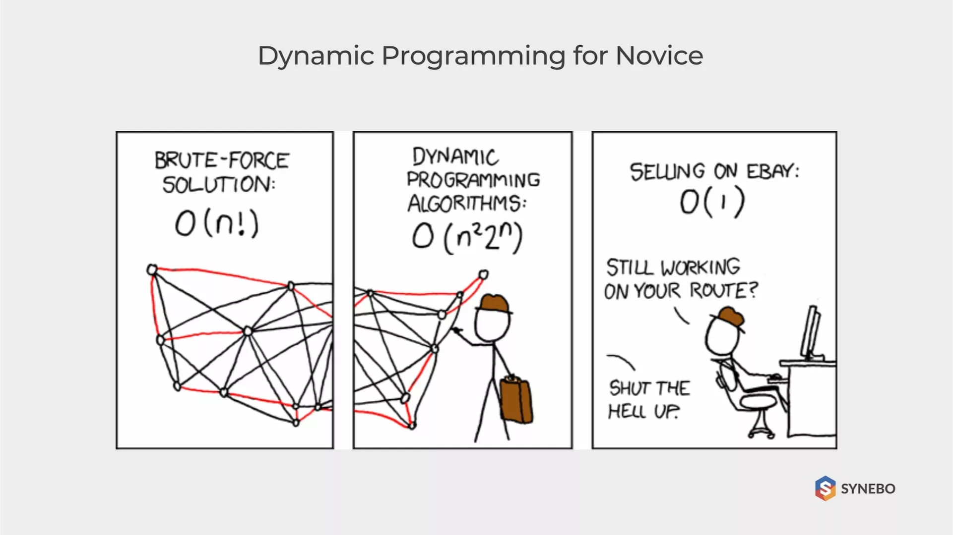
How to describe dynamic programming… Well, it is when we have a task that is quite incomprehensible. Therefore, we divide it into smaller tasks… which are also incomprehensible.
Dynamic programming is an algorithmic technique for solving problems based on a recurrent formula and a set of starting states.
Sub-solutions to the problem are formulated from those found in earlier steps. The most pleasant thing about this technique is that the solution has a faster polynomial complexity than naive methods (brute-force).
If you need experienced developers to handle Salesforce migration, integration, or other task, don’t hesitate to reach out to Synebo.
History of Dynamic Programming
The first association with dynamic programming is olympiad programming. Even though the method was tested in solving economic problems by Richard Belman for the first time, Belman (mathematician) formulated this approach to mathematical optimization and all the necessary conditions for applicability in difficulties.
The original version considered planning a multi-period production process at tiny steps and time points. Step by step, it was required to keep track of how the decisions made in production at previous actions reflected on the company’s further success and what to do next not to fail: buy a factory, sell timber, go offshore.
The optimality principle of Belman sounds like: the optimal policy has the property that regardless of initial states and initial decisions are taken, the remaining solutions should represent the optimal policy concerning the state resulting from the first solution. Hence, it’s also called the optimal substructure
Dynamic Programming Problems
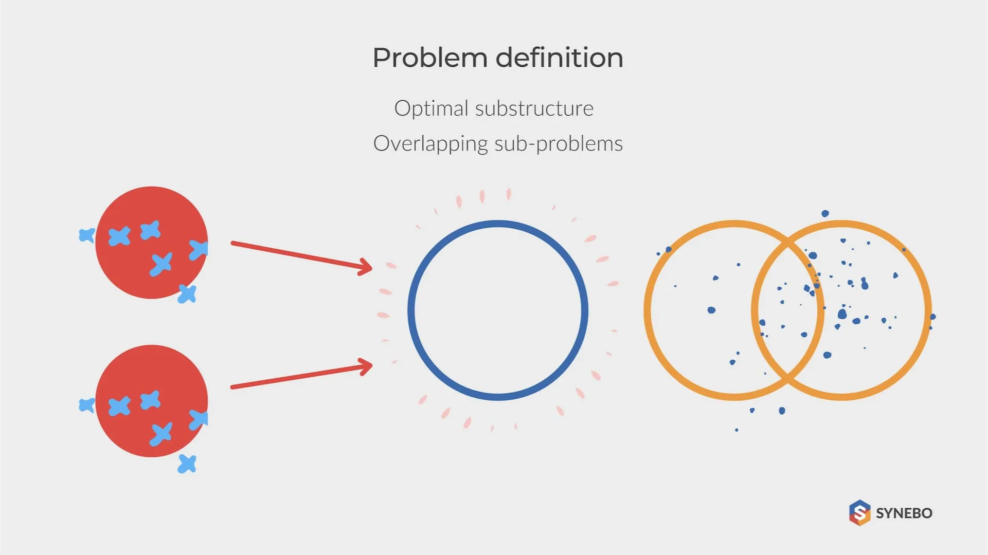
The problem has an optimal substructure if its optimal solution can be rationally compiled from the optimal solutions of its subtasks. The presence of the optimal substructure in the issue is used to determine the applicability of dynamic programming and greedy algorithms for solving this problem.
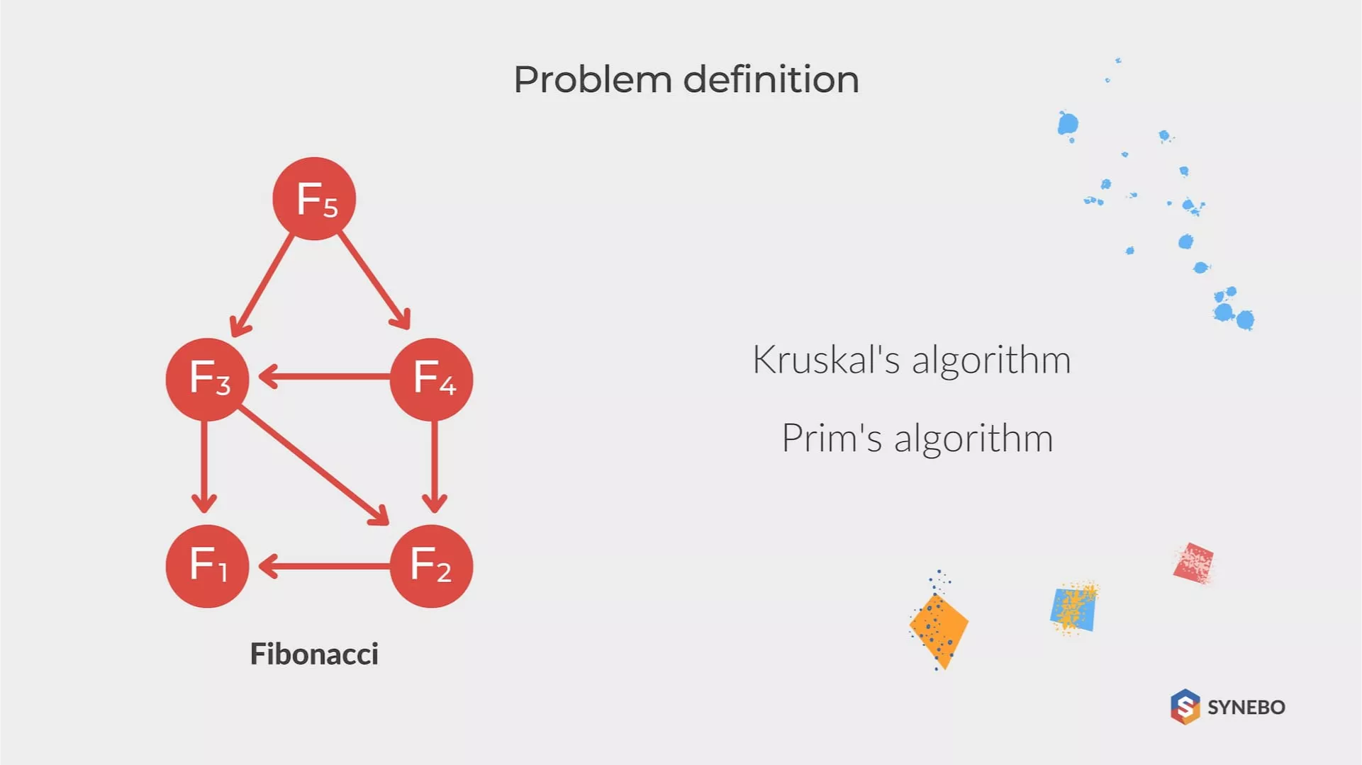
For example, the problem of finding the shortest path between some vertices of a graph contains an optimal solution of subtasks. Many problems solved by dynamic programming can be defined as searching in a given oriented acyclic graph of the shortest path from one vertex to another.
Depending on the formulation of the problem, whether dynamic programming on a segment, on a prefix, on a tree, the optimality term for subproblems can be different. But it is generally formulated as follows: if there is an optimal solution for some subtask that arises in solving the problem, then it should be used to solve the problem in general.
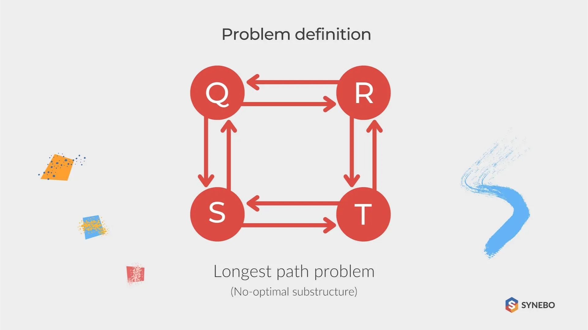
During the process of compiling dynamic programming algorithms, it is required to follow a sequence of four actions:
- First, describe the structure of the optimal solution.
- Recursively determine the value of the optimal solution.
- Calculate the value of the optimal solution using the method of bottom-up analysis.
- Make an optimal decision based on the received information.
Dependence of the elements of dynamics can be directly given in a condition (this usually happens if this is a problem for numerical sequences). Otherwise, you may find some known number series (like Fibonacci numbers) by manually calculating the first few values. If you are not lucky, you will have to think.
Are you interested in exploring how to send emails via Outlook API from Salesforce Org? Read another our guide.
Recurring Formulas
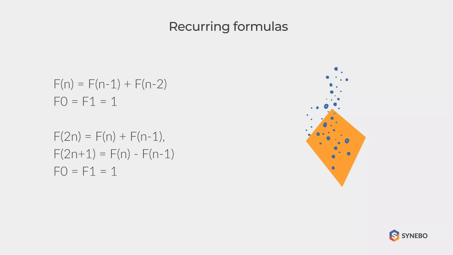
Given: initial states (a0 = a1 = 1), and dependencies. The only difficulty that can arise is the understanding that 2n is a parity condition for a number, and 2n + 1 is an odd number. Basically, we need to check whether the number is even and make calculations according to different formulas.
Recursion Vs. Loop
The recursion or cycle is a constant problem of choice when implementing the algorithm for a solution. The recursion arises from the condition of the problem (a repeating formula, etc.). Usually, it works perfectly, and you can implement it quickly and easily.
Sequential computation
Now let’s get back to where we started – the recursion is slow. It’s not too slow to bring real troubles, but it might become a problem in tasks where every millisecond is critical.
The main but not the only drawback of the method of sequential computation is that it is suitable only if the function refers exclusively to the elements in front of it. Our problem satisfies this condition.
The essence of the method is as follows: we create an array of N elements and sequentially fill it with values.
Recursive Solution with Value Caching
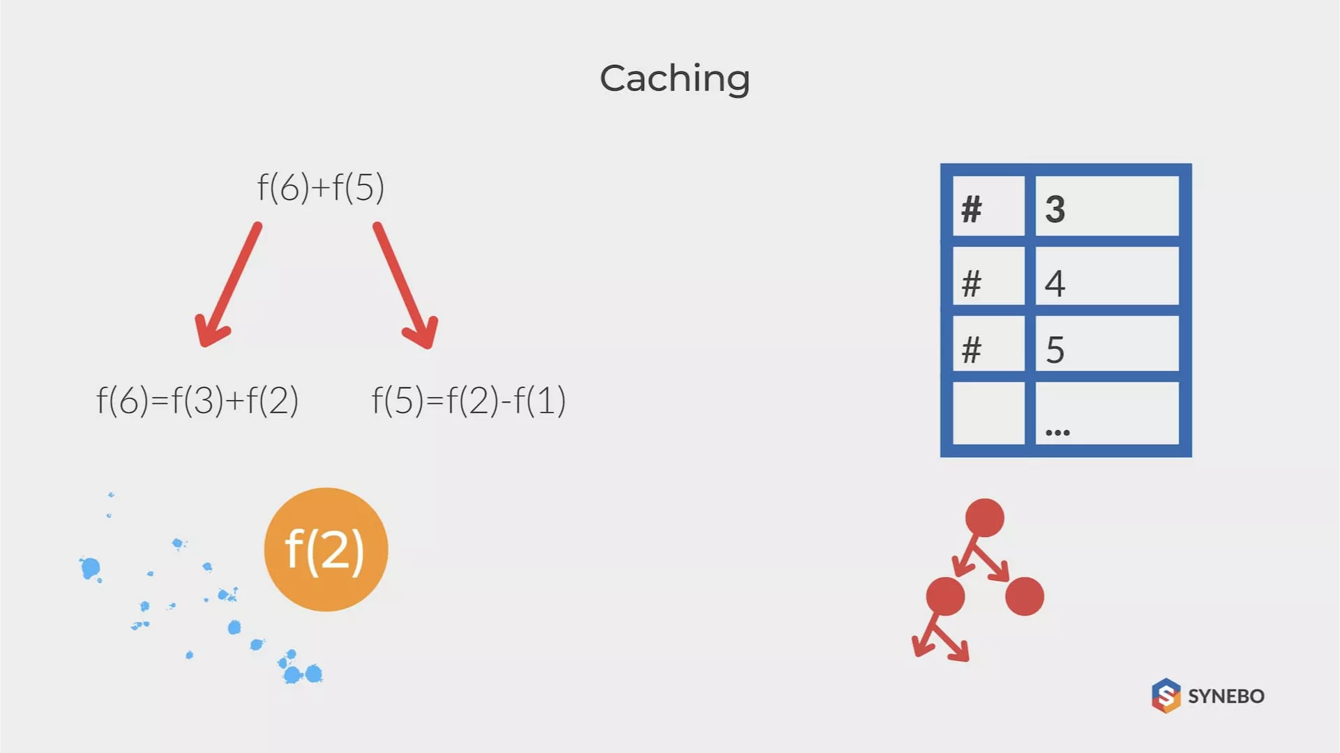
The idea of memoization is elementary – once calculating the value, we put it in some data structure. Then, before each calculation, we check whether a computed value is presented in this structure, and if it is there, we use it.
You may use an array filled with flag values as the data structure. However, if the element value by the index N is equal to the flag’s value, then we probably have not calculated it yet. This creates particular difficulties because the value of the flag should not belong to the set of values of the function, which is not always obvious.
A hash table is a good choice – all actions in it are performed for O (1), which is very convenient. However, two numbers can have the same hash with many values, which, naturally, causes problems. In this case, it is worth using, for example, an RB tree.
Typical Task
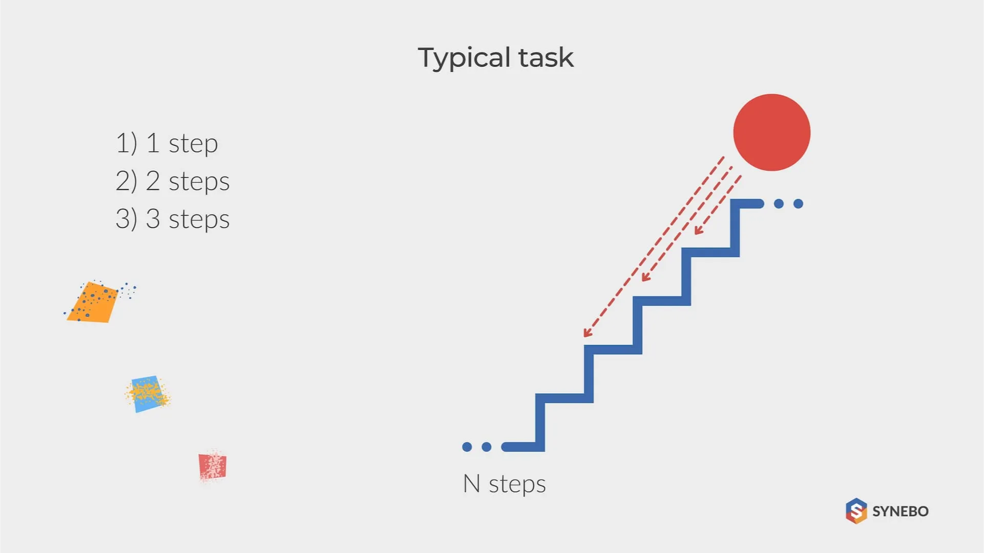
A ball starts jumping down to the bottom at the top of the ladder, containing N steps. The ball can jump to the next step or jump over one or two steps. (for instance, if the ball is on the 8th step, it can move to the 5th, 6th, or 7th.) First, determine the number of possible “routes” of the ball from the top to the ground.
The idea of a solution. The first step can be accessed only by making a jump with a length equal to one. The second step can be reached by jumping to 2 or only two options from the first step. Finally, the third step can be reached by jumping three, from the first or second.
Specifically, there are only four options (0-> 3; 0-> 1-> 3; 0-> 2-> 3; 0-> 1-> 2-> 3). Considering the fourth step, you can get there from the first step – one route for each route to it, with the second or third – the same. In other words, the number of ways to the 4th step is the sum of the routes to the 1st, 2nd, and 3rd steps. Mathematically, F (N) = F (N-1) + F (N-2) + F (N-3).
2-d Dynamic
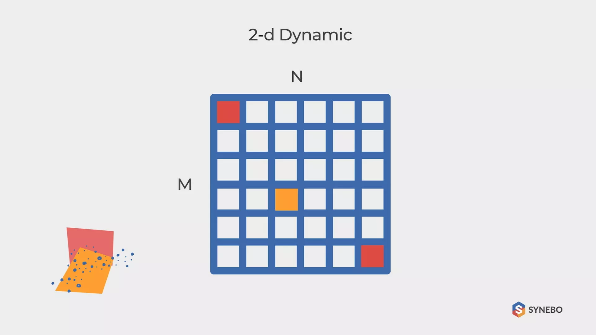
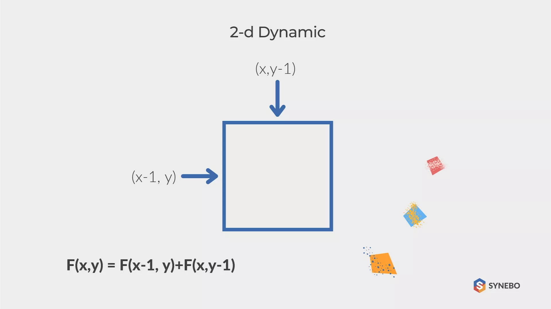
In the rectangular table NxM in the beginning, the player is in the left upper cell. They’re allowed to move to the next cell in one move, either to the right or down. However, it is forbidden to move to the left and upwards). So you have to calculate how many ways a player has to get to the right lower cell.
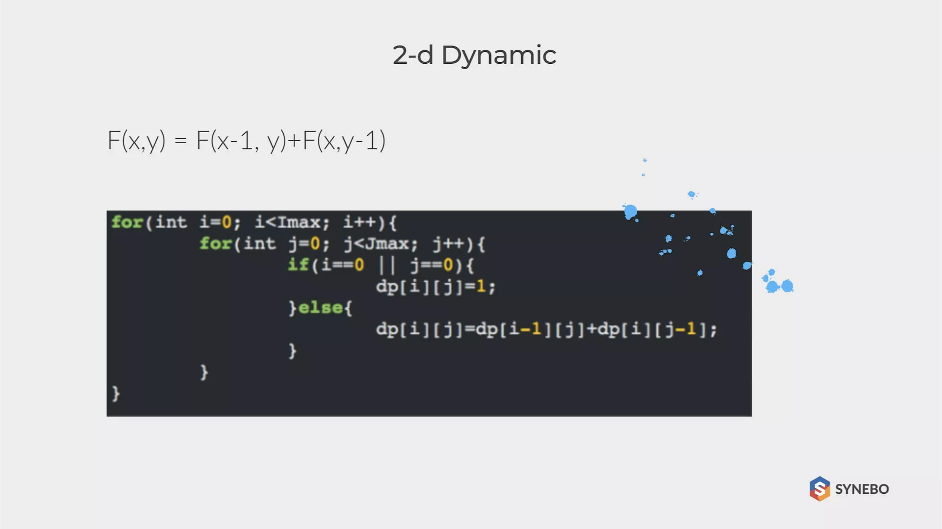
The logic of the solution is completely identical to the problem with the ball and ladder – but now it is possible to get into the cell (x, y) from cells (x-1, y) or (x, y-1). Totally F (x, y) = F (x-1, y) + F (x, y-1). In addition, it is possible to understand that all cells with values (1, y) and (x, 1) have only one route, either straight down or straight to the right.
Are you in need of Salesforce consulting Services? Reach out to Synebo, an experienced provider of Salesforce services.
Explosion Hazard Task
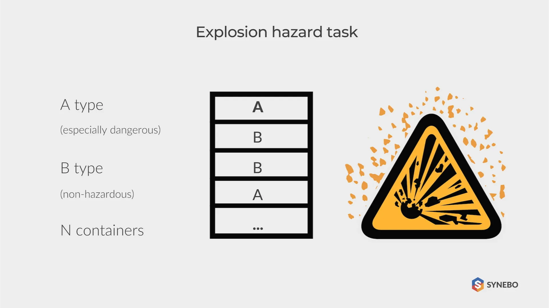
When processing radioactive materials, waste forms two types – hazardous (type A) and non-hazardous (type B). The same containers are used for their storage. After placing the waste in the containers, the latter are stacked in a vertical pile.
A stack is considered explosive if more than one type A container in a row. A stack is safe if it is not explosive. Determine the number of possible kinds of safe stacks for a given number of containers “N.”
The answer is (N + 1) – Fibonacci number. You could guess by simply calculating the first 2-3 values. Each primary element is divided into the main (ends with B) and the secondary (ends with A). Then, the side elements are transformed into basic ones (only B can be added to the sequence ending in A).
Broken Calculator Task
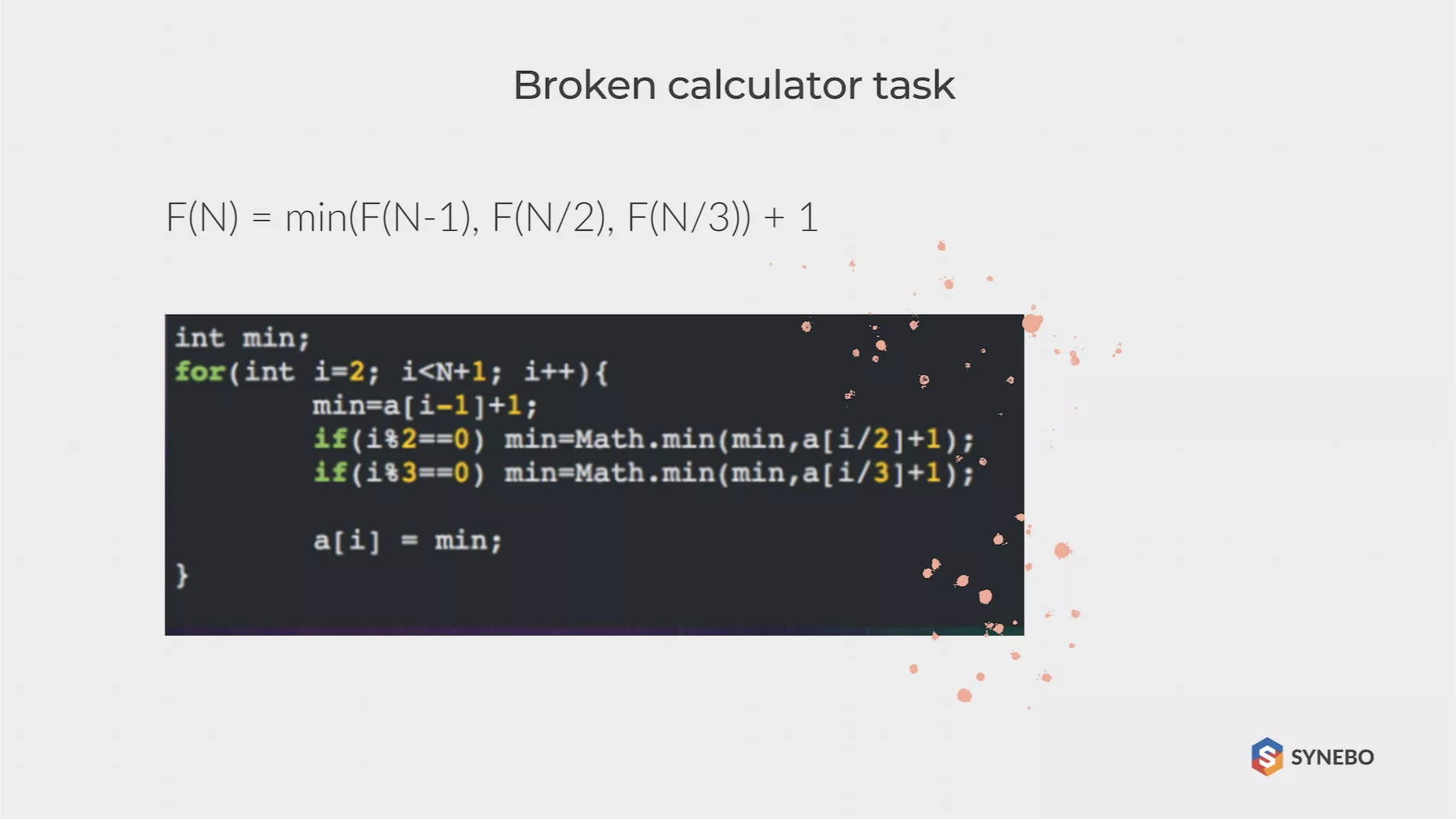
A calculator performs three operations: Add to the number X unit; Multiply X by 2; Multiply the number X by 3. First, determine: which least number of operations is needed to obtain “N” from a given number 1. Output this number, and, on the following line, a set of executed operations “111231”.
The naive solution is to divide the number by 3, as long as possible, otherwise by 2, if possible, subtract a unit, and so on until it turns into 1. However, this is a wrong decision because it excludes, for example, the possibility of reducing the number by one and then dividing by three, which causes errors with large numbers (for example, 32718).
The correct solution is to find for each number from 2 to N the minimum number of actions based on the previous elements, basically: F (N) = min (F (N-1), F (N / 2), F (N / 3) ) + 1. It would be best if you remembered that all indices must be integers.
To recreate the list of actions, you need to go in the opposite direction and look for index i when F (i) = F (N), where N is the number of elements in question. If i = N-1, put one at the beginning of the line. If i = N / 2 – put two; otherwise – three.
Golden Pyramid
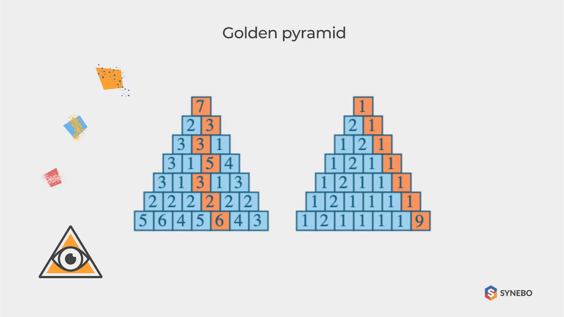
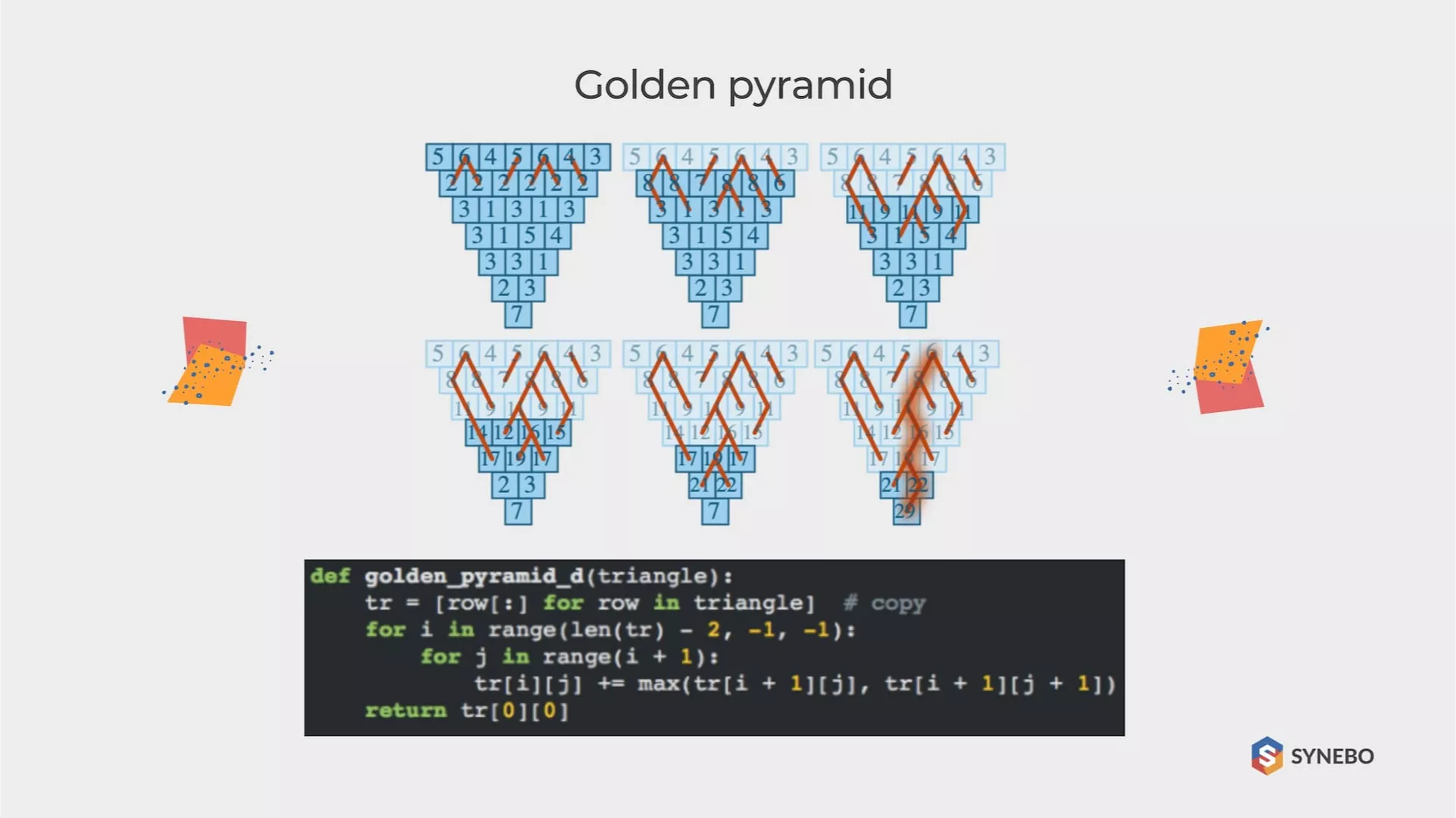
Imagine a triangle composed of numbers. One number is located at the top. There are two numbers below, then three, and the right to the bottom. So you start at the top, and you need to go down to the bottom of the triangle.
You can go one level down and choose between two numbers under the current position for each move. While walking this path, you “collect” and summarize the numbers you pass. Your goal is to find the maximum amount from different routes.
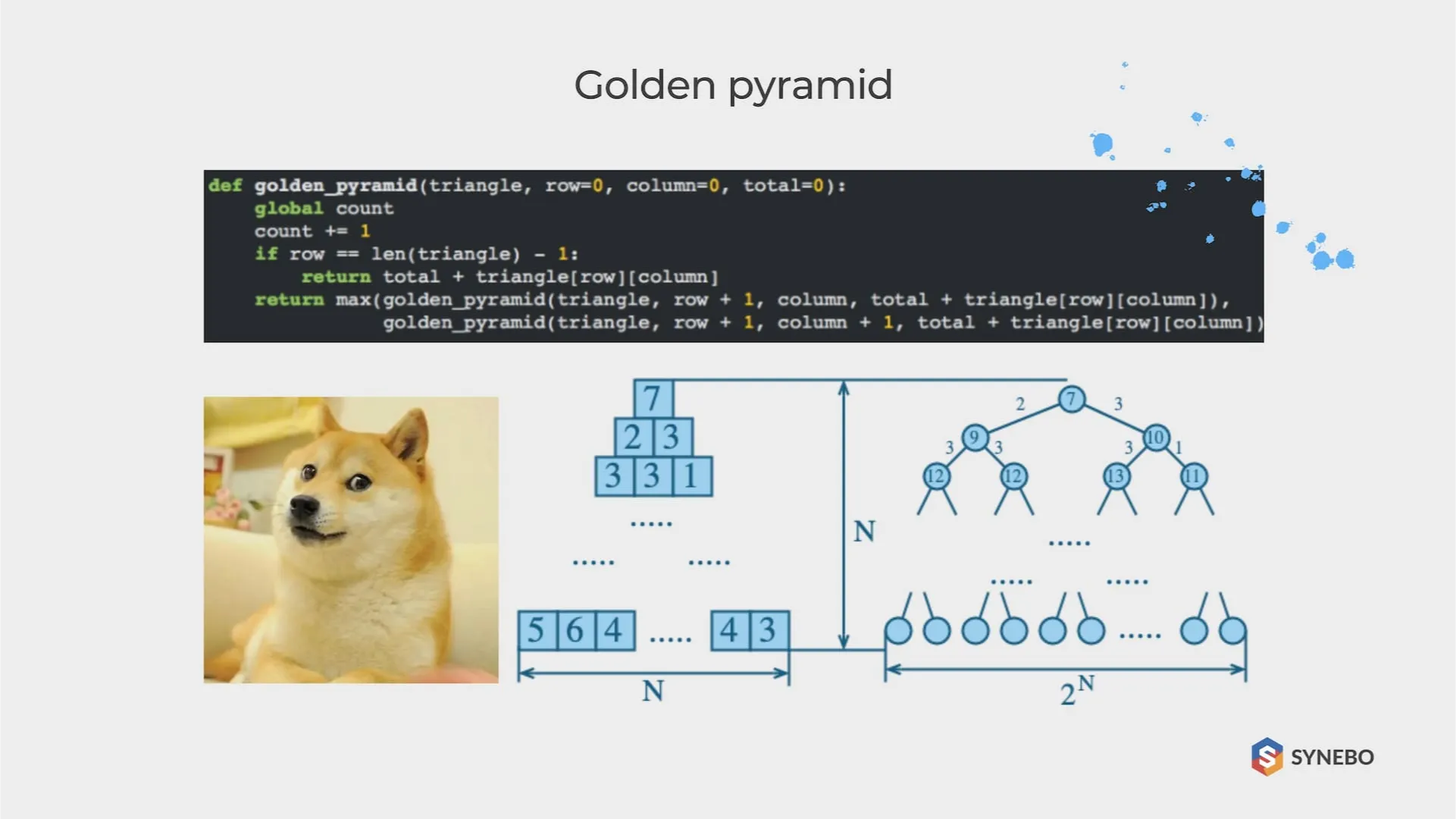
The first thing that comes to mind is using recursion and calculating all the paths from the top. Then, when we go one level down, all available numbers shape a new smaller triangle, and we can start our function for a new subset and continue this until we reach the bottom.
What if we try to use the principle of dynamic programming and break our problem into many small subtasks, the results of which we can accumulate afterwords. Try to look at the triangle upside down. And now to the second level (penultimate from the bottom).
We can decide the best choice for each cell in our small three-element triangles. Choose the best, summarize with the considered cell and write the result. After all, we will get our triangle, but one level lower.
Repeat this operation again and again. As a result, we need (N-1) + (N-2) + … 2 + 1 operations, and the algorithm’s complexity is N2.
Looking for a trusted provider to assist you with Salesforce development of any kind? Drop Synebo a line and let’s discuss!
What’s Next
A “greedy” algorithm, like dynamic programming, is applicable in those cases where the desired object is built from pieces. The “greedy” algorithm at each step, locally, makes an optimal choice.
A simple example is when trying to gain a certain amount by the minimum number of coins. You can consistently type coins with the maximum value (not exceeding the remaining amount). A “greedy” algorithm usually works much faster than an algorithm based on dynamic programming, but the final solution will not always be optimal.
Amortization analysis is a means of analyzing algorithms that produce a sequence of similar operations. Instead of evaluating the operating time for each operation separately, the depreciation analysis estimates the average operating time per transaction.
The difference can be significant if long-running operations are in progress. Depreciation analysis is not only a tool for evaluating algorithms but also an approach to development (this is closely related)
For more information, check our presentation here.
Use dynamic programming when a problem can be broken down into overlapping subproblems that can be solved independently. It’s particularly useful for optimization problems where a solution can be constructed from solutions to subproblems.
A dynamic programming algorithm is a method for solving complex problems by breaking them down into simpler subproblems, solving each subproblem once, and storing their solutions. It combines the solutions of the subproblems to solve the original problem efficiently.
To solve dynamic programming problems, first identify the subproblems by breaking down the main problem into smaller, overlapping subproblems. Then formulate a recursive solution to express the problem in terms of its subproblems. Use memoization or tabulation to store the solutions of subproblems to avoid redundant calculations. Finally, use the stored solutions to construct the solution for the original problem.


